|
|
Modeling the Edwards Aquifer
The first rule of modeling:
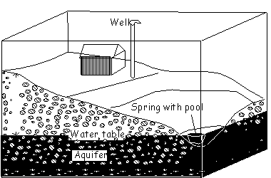
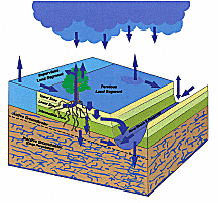
At their best, models can be used to help decision makers evaluate large, complex problems and determine an appropriate course of action. There are many different types of models. Simple physical models such as an aquifer built in an aquarium can help us understand how aquifers function and how they react to different things like rainfall or pollution. Virtual digital simulation models use computers to solve complicated mathematical equations, and they can allow water managers to explore the impacts of various conditions or management plans without actually doing anything that might reduce spring flows or harm endangered species. Complex digital computer simulations can also help us visualize the aquifer in three dimensions and understand how it works. Models may also take the form of financial spreadsheets that analyze costs and benefits. We are going to look at all these types of models here. Models are usually just one piece of a larger puzzle when we are looking at real-world problems from a systems analysis approach. Systems analysis is a philosophy of problem solving most often used with large, complex problems where a decision maker collects information and uses everything available to decide what to do. It is not a cookbook approach or a box where we insert data, turn a crank, and get an answer. There are basically three types of questions that modeling addresses, and systems analysis usually involves solution processes and modeling designed to get answers to questions of the third type:
Obviously, questions of the third type are the most difficult to
answer. Most of the models that have been developed for the Edwards
Aquifer mainly help to answer the first two questions; but they can be used in
conjunction with other systems analysis methods to help answer that difficult
third question. So far, none of the Edwards models have really been widely
used as management tools. Most of the existing models
are very complicated and difficult to use in everyday decision-making and
Aquifer management. There has always been concern that models are not calibrated
well enough to what
really happened in the past. Decision makers want to be certain the models are as fully developed
and as accurate as
they need to be before using them to make critical decisions. In addition,
there are people who don't like what the models suggest! For example, all the models that predict springflow tell basically the same story...
reductions in pumping can increase springflows but probably won't keep them flowing in an extreme drought.
One model goes a step further and points out the economic cost of reducing
pumpage is huge, yet springs still go dry. And the
bottom line is that no one really has a well developed, integrated surface-ground water hydrology
model that can be used as a conjunctive management tool. Another problem is that no one really has a good handle on what pumpage has been
historically for irrigation and industry. Municipal pumpage is easy to determine, but when it
comes to farming there’s a lot of variables and guesswork involved.
Still, decisions have to be made, and making decisions in the face of uncertainty, based on incomplete information but
using the best data you have, is the stuff of systems analysis.
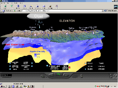
The Models: 1979 - Texas Water Development Board Finite-Difference Model (with 1992 refinements) 1983 - Discrete-State Compartment Model 1988 - United States Geological Survey Finite-Difference Model 1993 - A & M University Economic / Hydrologic Model 1994 - United States Geological Survey Finite-Element Model 1995 - Edwards Underground Water District Edwards Aquifer Simulation 1999 - Bureau of Economic Geology 3D Virtual Reality Model 2004 - 3D Model of the Edwards in Northern Bexar County 2005 - HSPF Recharge Model for the San Antonio Segment of the Edwards Texas Water Development Board Finite-Difference Model In the mid-1970's, researchers at the Texas Water Development Board evaluated and synthesized previously compiled geologic and hydrologic data, collected additional data, and initiated synthesis and analysis studies using digital computer modeling techniques. These pioneers were William B. Klemt, Tommy R. Knowles, Glenward R. Elder, and Thomas W. Sieh. Their objectives were to investigate the influence of projected water demands on Aquifer storage and spring flow, to determine the effectiveness of artificial recharge, and to discover whether ground-water management could protect spring flow at Comal and San Marcos Springs. Their model simulates water levels and spring flows based on the physical constraints of the system and on the recharge and pumpage rates for the Aquifer.
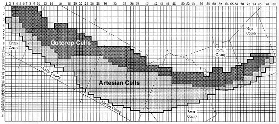
Finite Difference Grid for TWDB model
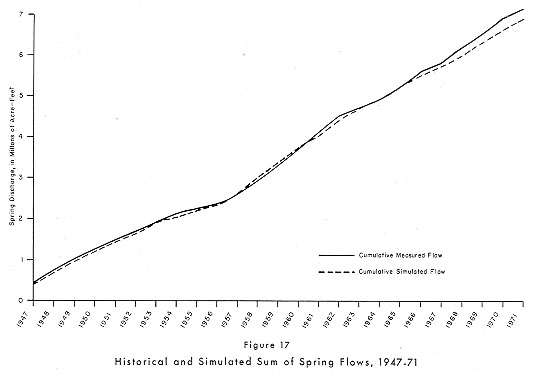
There are three types of cells in the model: outcrop cells, artesian cells, and boundary cells. In the graphic below, the boundary cells are the ones with at least one black, bold border; the outcrop cells are in dark grey; and the artesian cells are in light gray. Most of the grid cells lie outside the boundary, so only 856 of the cells in the grid were considered as part of the Edwards system and included in the simulation. Critical steps in model building are the assignment of recharge and pumpage values to each of the cells. Recharge was divided into two components: water that recharges by going down through sinkholes and faults in creek beds, and water that becomes recharge by falling directly onto the outcrop. In the assignment of recharge, the amount of water known to have been lost from a stream to recharge was assigned evenly to the cells that contained the stream reach, and the amount recharged by direct infiltration was evenly divided among the remaining cells for that subbasin. Assignment of pumpage is also critical - it must be assigned so it approximates the distribution of pumpage that actually occurred. In this model, the pumpage assigned to each cell is the total pumpage of all wells located within the cell. Model Calibration After a model is initially built, there comes a calibration phase that involves comparing observed and simulated water levels. The idea is to find out how well the model can predict what actually happened in the past. For this model, the calibration period used data from 1947 to 1971. This period was chosen because the data was readily available and these years included a great variation in water levels. There was an extreme drought that lasted from 1947 until 1956, and 1957 and 1958 were years of unusually high recharge. It was felt that if the model could simulate water levels for this period, it would be well calibrated. The calibration results are shown in the graphic below, and it is clear the measured flow and the simulated flow are very close. The difference amounts to only 4.3 percent of the total flow. Based on this comparison, it was decided the digital model was calibrated to a degree of accuracy sufficient to reproduce past events and that the model could therefore be used to predict future Aquifer conditions as a tool in evaluating and developing management plans.
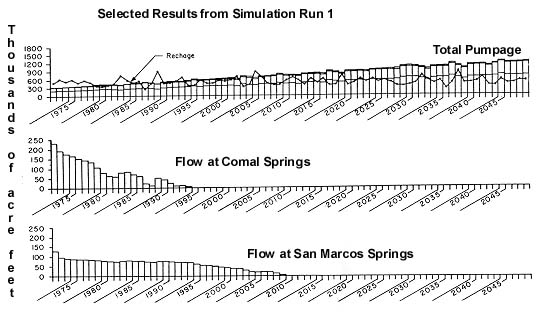
After calibration, a Future Simulation Phase involved using the model to predict what would happen in the Aquifer under a variety of different conditions. There were a total of 20 model runs that looked at the response of the Aquifer under a variety of pumpage and recharge conditions, various drought and flood conditions, several Aquifer management plans, and under augmentation pumping. Below are some selected results from Simulation Run 1. By the year 2000, total Aquifer pumpage was projected to be around 650,000 acre-feet. Comal Springs was projected to go dry in 1995, and San Marcos Springs would be dry by 2010. Pumpage has not really panned out as was projected back in the 70's when this model was built. Currently there is a cap on pumpage at 450,000 acre feet, and the Springs are still flowing.
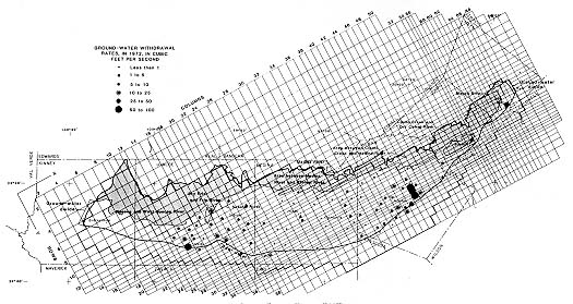
The 20 model runs suggested the Aquifer could indeed meet the demand projections, but the natural flow of Comal and San Marcos Springs would cease by 2020 if projected pumpage occurred as predicted. It also concluded the addition of artificial recharge that was being proposed at the time did not result in an appreciable increase in the Aquifer's available water. Further, it suggested the drought-flood sequence of the 1950's produced only minor effects compared to the long-term influence of pumpage by humans. The model also concluded that spring flows at Comal and San Marcos Aprings could be maintained through groundwater management plans. Finally, it suggested there is sufficient storage in the Aquifer to allow spring flow of Comal and San Marcos Springs to be replaced by augmentation pumpage. 1992 Model Refinement In 1992, David Thorkildsen and Paul D. McElhaney revisited the 1970's model, refined it, and applied it under new conditions of reduced regional pumpage and under new Aquifer management plans. During the years between 1979 and 1992, the United States Geological Survey continued to collect new and better data on things like Aquifer transmissivity, storage coefficients, and anistropy, so these two geologists at the TWDB were able to incorporate the new data into their model to better represent the flow system and improve the model simulation. For the new version of the model, the time period used for calibration was 1947 to 1959 instead of 1947 to 1971 as before. It was thought that since this period was one of extreme stress that included a major drought and a recovery period, it would be a good test for the parameters in the model. The time step for output results became monthly instead of annually. After calibration, the model was used to simulate Aquifer response to several constant pumpage scenarios under recharge conditions of the drought and recovery sequence (1947-1959). The results indicated that large pumpage reductions would be necessary in order to ensure minimum springflows in the 40 to 50 cfs range at both San Marcos and Comal Springs. For a flow of 50 cfs or greater to be maintained at Comal Springs, the model indicated total pumpage would have to be in the 225,000 to 250,000 acre-feet per year range for the entire San Antonio region. This is much less than current pumpage. To maintain 100 cfs or greater, the model indicated maximum total pumpage would be about 165,000 acre feet per year. The model also looked at the effect of reduced pumpage in the western, agricultural part of the Edwards region. Interestingly, the model indicated this would result in an increase in springflow at Comal Springs, but the increase was not equal to the amount of pumpage reduced. If the reduction in pumpage was placed in Uvalde county, only 34% of the reduction shows up as springflow at Comal Springs after nine years. If the reduction was placed in Medina county, 67% of the reduction was seen as increased springflow at Comal Springs after nine years. In both cases the remainder of the reduced pumpage either became increased Aquifer storage, interformational flow, or increased outflow. When the reductions were placed in Uvalde county, Leona springs began to flow again; but not when the reductions were placed in Medina county. One of the ideas being floated in the early 90's by the Texas Water Commission was a mandatory water curtailment plan called the "dry-year option", under which pumpage for municipal, industrial, and aquaculture was adjusted (decreased or increased) on a monthly basis based on the simulated water level in the model cell representing the J17 monitoring well. Irrigation pumpage was to be adjusted on an annual basis, also using the simulated water level at J17. Under this plan, the model indicated that San Marcos Springs would always flow, but Comal Springs would cease to flow in an extreme drought. UTSA's Decision Support System In the mid-90's the University of Texas at San Antonio built something called the Decision Support System for the Edwards. It was actually the TWDB model converted to run on a personal computer, with minor embellishments and additions. This was the first model that had an interface sufficiently developed that a water manager could use it behind a desk. It has not been widely used outside academic circles. United States Geological Survey Finite Difference Model In 1988, Robert.W. Maclay and L.F. Land, working for the United States Geological Survey, developed an Edwards model that focused on concepts such as the effects of barrier faults and storage within the aquifer. Like the TWDB model, it was a finite-difference model, but it was modified to provide the capability of representing barrier faults. Rather than predicting Aquifer levels under different conditions as in the TWDB model, the main objective was to learn more about storage of water in different parts of the Aquifer and identification of flowpaths within the aquifer. Finite Difference Grid for USGS model
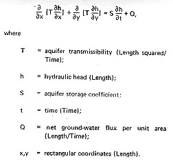
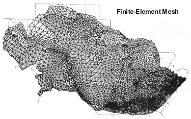
The important thing to notice about this grid is the orientation is about 65 degrees east of north. This was done to achieve the best alignment with the faults west of Cibolo Creek. The math model assumes that one of the x,y Cartesian coordinate axes is aligned along the principal component of the transmissivity. More than 300 simulations were performed, and the modeling effort resulted in several major interpretations. One significant interpretation was that two essentially independent areas of regional flow exist in the west and central portions of the Aquifer, and flows from the two areas converge at Comal springs. Barrier faults deflect patterns of groundwater movement, and the most noticeable deflection is the convergence of flow through a geologic structural opening, the Knippa Gap, in eastern Uvalde county. A second significant interpretation is that groundwater flow in northeastern Bexar, Comal, and Hays counties is diverted by barrier faults toward San Marcos Springs. The simulations showed that several barrier faults in the northwestern part of the San Antonio area had a significant effect on storage, water levels, and springflow within the Edwards Aquifer. A lumped parameter model for the Edwards was developed in 1992 by Nisai Wanakule and Roberto Anaya with funding from various agencies. Their objective was to develop and test a simple and easy to use model to accurately simulate monthly water levels and springflows of the Edwards Aquifer. The model was formulated using a discrete, nonlinear, non-stationary system based on control theory. The main advantage of this simulation model was that it could utilize limited data to provide accurate, short-term estimates of Aquifer levels and springflows. Previous models required massive amounts of inputs and generated only annual estimates. Basically, the Edwards Aquifer was represented as a series of connected rock-filled tanks that represent eight major drainage basins of the Aquifer and springflows at Comal and San Marcos springs. Individual drainage basins included the Nueces River, the Frio River, the Sabinal River, Upper and Lower Seco and Hondo Creek (these represent flows on both sides of the Knippa Gap), the Medina River, Helotes and Salado Creek, Cibolo Creek, and the Blanco River. Data from the Guadalupe River basin were not available and thus were not included. Inputs to the model included real time measurements of recharge from river gauging stations. Outputs of the model included forecasts of levels in seven key observation wells and springflows. The model estimates monthly recharge, water levels, and pumping in each basin. It also allows for the interaction of ground and surface water between sub-basins. Monthly stream gauge and Aquifer level data from 1975 to 1990 were used to calibrate the model, while data from 1962 to 1974 were analyzed to verify its performance. The simulation exercises showed the model is accurate and very easy to use because much less data is needed. When a Macintosh computer with a 68040 microprocessor was used, the lumped parameter model efficiently simulated 189 monthly iterations of water levels for nine drainage basins in less than four minutes. Recharge functions in the model provided good estimates of monthly recharge. Recharge estimates were very similar to results from the USGS model in most cases, although peak years were under-represented. For a long time this model was available to actually be run on the web by any interested person. A & M University Economic / Hydrologic Model In 1993, Bruce McCarl and Lonnie Jones of the Texas A & M University Agricultural Economics Department worked with graduate students R. Lynn Williams and Carl Dillon to investigate the implications of management plans that were being proposed for the Aquifer at the time. At that time, hardly any research had been done that looked at the effect of different management plans on the regional economy. In 1992, two management plans were drafted by the Texas Water Commission. The "Sector Plan" proposed specific cutbacks for agricultural, municipal, and industrial users when Aquifer levels at the J17 index well dropped to key levels, and the "Total Limit Plan" called for a total reduction in water use, but didn't specify where the cutbacks had to occur. Neither plan was adopted, but the Texas Legislature began considering plans similar to the TWC plans. A study was undertaken to evaluate the hydrologic and economic implications of the TWC plans. The A & M researchers analyzed four variants of the plans using an annual economic/hydrologic simulation model. The model simulated water use by the agricultural, industrial and municipal sectors while simultaneously forecasting annual spring flow and year-end water elevations. The model also accounted for uncertainty in recharge amounts and in the incidence of elevation-triggered pumping limits. A key feature of the model was that it optimized optimize water allocations among the various sectors of users based on maximizing economic welfare. In other words, water was allocated to the activities that generated the greatest economic value. The model suggested that the simultaneous imposition of pumpage limits, water rights and water markets would be necessary to maintain economic efficiency. To allocate water toward the highest value use, the model made the assumption that low valued users would allow high value user to use their water instead. In reality, this would be highly unlikely without compensation for the low valued users. So, a rights structure was also examined where the irrigated agriculture sector (generally a low valued user) was guaranteed water usage at their 1988 level. The model showed that under these circumstances, there are gains in agricultural welfare, but municipal, industrial and total welfare is reduced by more than the agricultural gain. And without an agricultural guarantee for an allocation at their 1988 level, the municipal and industrial gains are achieved at agriculture's expense. Either way, the model suggested everyone loses out economically when pumping is no longer unrestricted and water is allocated. It indicated the management plans were likely to result in annual losses for current water users ranging from $0.73 million to $1.5 million (based on 1988 demands), rising to $2.3 to $6.7 million in the year 2000. When the value of water is optimized in an economic sense, the model predicted an annual loss in regional economic activity of between $6.26 and $19.58 per acre foot that pumpage is reduced. By the year 2000, agricultural use value was equal to about $19 per acre foot while non-agricultural values were about $109 per acre foot. This suggested that paying farmers not to use water would make economic sense. The benefits of the management plans that were being proposed were increased flows at Comal and San Marcos Springs and higher year-end Aquifer levels. This model was the first attempt to quantify the economic cost of keeping springs flowing. It suggested costs would be very high, and there would still be no guarantee that Comal Springs would keep flowing in a severe drought. United States Geological Survey Finite-Element Model In 1994, Eve Kuniansky and Kelly Holligan, working for the United States Geological Survey, published a model that sought to understand and describe the regional flow system and examine how the Edwards Aquifer is connected to the Trinity Aquifer and other hydraulically connected units. The researchers wanted to gain a better understanding of how much water enters the Edwards from other Aquifers and how anistropy affects regional flows of groundwater. Anistropy occurs when water can move more easily through the rock matrix in one direction than another. In most Aquifers made up of flat-lying sedimentary rocks, water can move more easily horizontally than vertically. Because of this property, and because the Aquifer is many times wider than it is deep, groundwater flow through the Aquifer can be approximated with two dimensions even though the Aquifer actually exists in three dimensions. Unlike the previous models that used a finite-difference approach, this model used a finite-element method because it is one of the few numerical methods that can approximate anistropy.
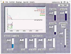
In this model, the major departure from the earlier simulations was this one allowed a hydraulic connection from the Trinity Aquifer. The previous models assumed a no-flow boundary between the Edwards and the Trinity. Two simulations were performed. One was for the winter of 1974-1975 because there was adequate water-level data for model calibration for that period; and the other simulation was for predevelopment conditions. The simulations indicated that a significant amount of water enters the Balcones Fault Zone from other aquifers; about 97,500 acre-ft per from the Trinity and an additional 292,500 acre-ft per year from the Edwards-Trinity Plateau aquifer west of the Haby Crossing fault. Also, large irrigation withdrawals from the Edwards-Trinity Aquifer and the Cenozoic Pecos alluvial Aquifer in the Trans Pecos region have resulted in the drying up of several springs including Comanche and Leon Springs. Further, the results also suggested that anistropy is an important factor in groundwater movement in the Balcones Fault Zone. In 1995 the Edwards Aquifer Simulation (EAS) was developed under the guidance of the Edwards Underground Water District. It was designed as an interactive tool to explore both the natural processes that influence and control the operation of the Aquifer and the human exploitation and management of the aquifer. It used a hands-on, role-playing environment that allowed users to model Aquifer response and springflows under many different scenarios such as varying rainfall patterns, institution of pumping restrictions, allocation of supply, and establishment of conservation and reuse programs. Unfortunately, this simulation was built for the Macintosh platform, so there were not many that could run it.
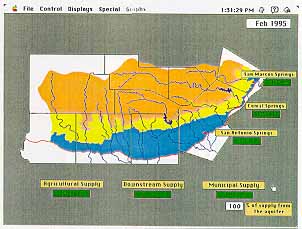
These are the two main display screens for the Edwards Aquifer Simulator. The Regional Map screen, at left, displays status indicators for springflow, municipal and agricultural pumpage, and downstream flow. The display would update annually during a model run. On the right, the Monitor Board screen displays graphical and numerical indicators of water level. Bureau of Economic Geology 3D Virtual Reality Model
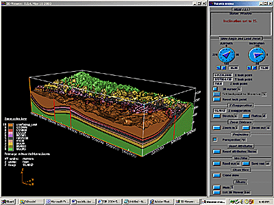
3D Model of the Edwards in Northern Bexar County
This model will on many platforms, including Linux, and it is a very cool tool for visualizing the structure of the Edwards in Bexar county. It is available from the USGS website at: http://pubs.usgs.gov/sir/2004/5226/ HSPF Recharge Model for the San Antonio Segment of the Edwards
In 2005 LB-Guyton
Associates, working for the Edwards Aquifer Authority, published a report
on their development of nine models for basins that recharge the San
Antonio segment of the Edwards. They used HSPF (Hydrologic Simulation
Program-Fortran), a popular and flexible modeling tool first developed in
the early 1960s that simulates the hydrologic processes, and associated
water quality, on pervious and impervious land surfaces and in streams and
well-mixed impoundments. HSPF can be adapted for almost any modeling task,
and it contains hundreds of process algorithms developed from theory,
laboratory experiments, and empirical relations from instrumented
watersheds. The most productive and easiest way to run HSPF is from a DOS
prompt, using structured input and output text files, so this model is
pretty much for computer geeks only.
The results indicated that total recharge estimates from the HSPF models are generally comparable to traditional methods used by the USGS and HDR. However, the recharge estimates for some basins are higher than previous estimates and others are lower. For the San Antonio River basin, the cumulative recharge estimates are slightly lower than estimated by the USGS and HDR methods, and for the Guadalupe basin they were slightly higher. For the western basins including the Nueces, Frio, Sabinal, and Sabinal-Medina, the cumulative recharge fell between the USGS and HDR estimates.
The model also suggested
that the source of recharge varies dramatically among the basins depending
on the channel loss characteristics, areal extent of recharge zone, and
volume of upstream flows from the contributing zone. In some basins, land
recharge is a major component of overall recharge and in other basins
recharge is dominated by channel loss. One of the most sensitive
parameters in the model was the channel loss in streambeds over the
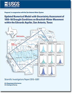
recharge zone. USGS Updated Numerical Model with Uncertainty Assessment of 1950-56 Drought Conditions on Brackish-Water Movement with the Edwards Aquifer In cooperation with the San Antonio Water System, the United States Geological Survey developed a new model with a focus on simulating the interaction between freshwater and saline water where they mix in the area called the brackish-water transition zone. The model results indicate that effects on fresh water during a severe drought would be minor. USGS scientist Linzy Brakefield said "While the model shows little potential for movement of brackish water into freshwater, the research suggests there is a need for an improved understanding of some parts of the Edwards Aquifer flow system. Better knowledge of how the Aquifer is recharged and the relationship between recharge, pumping, and springflow is needed. With the new developments from this study there is potential to develop more accurate models in the future."
|
||||||||||||||||||
|
Materials used to prepare this section: Edwards Underground Water District, (1995). Edwards Aquifer Simulator, Version 2 for Macintosh, User Manual. New Braunfels: TBEE Educational Consultants. Klemt, William B., Knowles, Tommy R., Elder, Glenward R., and Sieh, Thomas W. (1979). Ground-Water Resources and Model Applications for the Edwards (Balcones Fault Zone) Aquifer in the San Antonio Region, Texas. Austin: Texas Department of Water Resources, Report 239. Kuniansky, Eve L., and Holligan, Kelly Q. (1994). Simulations of Flow in the Edwards-Trinity Aquifer System and Contiguous Hydraulically Connected Units, West-Central Texas. Austin: US Geological Survey, Water-Resources Investigations Report 93-4039. LBJ-Guyton Associates, (2005). HSPF Recharge Models for the San Antonio Segment of the Balcones Fault Zone Edwards Aquifer. EAA Contract 02-87-AS McCarl, Bruce A., Jordan, Wayne R., Williams, R. Lynne, Jones, Lonnie L., and Dillon, Carl R. (1993). Economic and Hydrologic Implications of Proposed Edwards Aquifer Management Plans. College Station: Texas Water Resources Institute, Technical Report No. 158. Maclay, R. W., and Land. L. F. (1988). Simulation of Flow in the Edwards Aquifer, San Antonio Region, Texas, and Refinement of Storage and Flow Concepts. Washington: US Government Printing Office, US Geological Survey Water-Supply Paper 2336-A. Pantea, Michael P. and Cole, James C. (2004). Three-Dimensional Geologic Framework Modeling of Faulted Hydrostratigraphic Units within the Edwards Aquifer, Northern Bexar County, Texas. USGS Scientific Investigations Report 2004–5226. Thorkildsen, David and McElhaney, Paul D. (1992). Model Refinement and Applications for the Edwards (Balcones Fault Zone) Aquifer in the San Antonio Region. Austin: Texas Water Development Board, Report 340. Wanakule, Nisai, and Anaya, Roberto (1993). A Lumped Parameter Model for the Edwards Aquifer. College Station: Texas Water Resources Institute, Technical Report No. 163. |
